LAB SESSION 7

LAB SESSION 7

NORMAL APPROXIMATION OF THE BINOMIAL

INTRODUCTION: The normal distribution is one of the most important distribution functions in statistics. We will now see how the binomial probabilities can be reasonably estimated by using the normal probability distribution. Later we will need to determine whether normality is a reasonable assumption. We will start our investigation with a few specific binomial distributions.

Step 1:Entering the data. For this demonstration we will use columns A, D, and G to hold a series of numbers. The corresponding probabilities will be placed into B, E and H. Enter the numbers 0, 1, 2, 3, and 4 into column A. Similarly, set D to the numbers 0, 1, ..., 8 and to set G to the numbers 0, 1, 2, ..., 24. These three columns will be used for three specific situations: n = 4, n = 8, and n = 24.

Step 2:Calculating and Storing the Probabilties. We will now place the binomial probabilities for A into B using BINOMDIST with n = 4 and p = .5.

Reminder on how to do this from Lab #6: Activate cell B1 and continue with:

Choose: Insert function, f_x > Statistical > BINOMDIST > OK

Enter: Number_s: A1:A5, or select cells

Trials: 4

Probability_s: .5

Cumulative: false > OK

Drag: fill handle down to give other probabilities

Place the binomial probabilities for D into E and G into H, being sure to use n = 8 and n = 24, respectively (keep p = 0.5.)

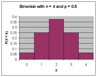
Step 3:Plotting the Probabilities Now we will plot each of the probabilities of x for 0 to n for n = 4 by using the Chart Wizard and procedures identical to earlier constructions of charts:

Select cells to be used for the chart

Enter: ChartWizard > 1st picture > Next

Select: the Series tab

Activate: Category (x) axis labels: select appropriate cells (A1:A5) > Next

Enter: appropriate titles > Next > Finish

Chart can then be modified to remove the gaps

Repeat this procedure for plotting E versus D and H versus G. What can we say about the distribution as n becomes larger?

Step 4:Interpreting the results.

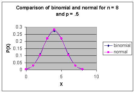
Let's see how the normal distribution approximates a binomial with p = .5 and n = 8. The approximating normal distribution has mean mu = 8(.5) = 4 and standard deviation sigma = sqrt((8)(.5)(.5)) = 1.414

First, we need to place the normal probabilities for each x (column D) into another column, say column F.

Activate cell F1 and enter: =NORMDIST(D1:D9, 4 ,SQRT(8*.5*.5),FALSE)

Click and drag: fill handle to generate normal probability for each x

To draw the graph of a the normal probability curve along with a binomial

probability curve, activate cells D1 through F9, then continue with

Choose: Chart Wizard > XY (Scatter) > 2nd picture > Next

Select: the series tab and enter binomial for the name of series 1, then

click on series 2 and enter the name normal > Next

Select: the titles tab and enter appropriate titles > Next > Finish

The chart just executed plotted the probability distribution function for the binomial and for the normal approximation on the same axes. This will help us see why we can approximate a binomial by a normal and how to do the appropriate calculations.

You should visualize the histogram corresponding to the binomial probabilities. The height of a bar is the probability the binomial variable is equal to the corresponding value. For example, the height of the bar centered at 5 is the probability the binomial is equal to 5. The base of a bar is 1 unit wide. Therefore, the area of a bar is equal to its height, and is thus equal to the corresponding probability.

Also visualize the normal curve.

Here are some calculations that will help the explanation. Suppose we want the probability that the binomial variable has a value from 5 to 7. This probability is the sum of the probabilities at 5, 6, and 7. (Look in Rows 6, 7 and 8 in column E: the sum is 0.359375) The area under the normal curve that goes from 4.5 to 7.5 approximates the area of the three binomial bars. How could we determine this area?

The probability the binomial variable has a value from 5 to 7 is .359375 . The approximation obtained from the normal probability distribution is .353205 without continuity correction, which is very close to the true probability. If we were to use a normal approximation for a binomial with p = .5 and n = 24 (like in columns G and H), the approximation would look even better. In the exercises, we'll look at other values of p.

ASSIGNMENT:

1. (a) Make plots as in the first part of the lab, but use p = .4 instead of p = .5.

Use n = 4, 8 and 24.

(b) Repeat part (a) using p = .2.

For what values of n and p does it seem to work best?

2. Suppose X has a binomial distribution with p = .8 and n = 25. Use Excel to calculate each of the probabilities below exactly. Also compute the normal approximation to these probabilities. Compare the binomial results with the normal approximations.

(a) P(X = 21)

(b) P(X < 21)

(d) P(21 < X < 24)

3. Do Exercises 6.83 and 6.85 in your text