LAB SESSION 16
LINEAR REGRESSION ANALYSIS
INTRODUCTION: In an earlier lab, we looked at bivariate
data, and used the linear correlation coefficient to see if there was a
relationship between the two variables.
You also looked at a method of developing a line of best fit. In this lab we will look at a method of
deciding whether the equation of that line is of any use to us in making point
predictions and developing confidence intervals.
Before
beginning this lab, you should review the commands for performing a regression
analysis in Lab 5. Use the data in
Exercise 13.33 just to refresh your memory.
Enter x values in column A (independent variable)
Enter y values in column B
(dependant variable)
Choose: Tools>Data
Analysis>Regression OK
Enter: Input y range: B1: B11 (or select cells)
Input X
range; A1:A11 ( or select cells)
Select:
Labels (if you labeled your columns)
Confidence level: 95% (or desired level)
Select:
Output Range: C3 (or upper left corner of where you
want
output to appear)
Check the
following boxes, depending on desired output:
Residuals:
to obtain predicted values and their
residuals
Residual
Plots: scatterplot of residuals against their x values
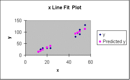
Line Fit
Plots: scatterplot of y against x
Note: You
can make the output nicer looking if you choose
Format>Column>Autofit
|
|
|
|
|
|
|
|
|
|
|
|
|
|
|
|
|
|
|
|
|
|
|
SUMMARY
OUTPUT |
|
|
|
|
|
|
|
||
|
|
|
|
|
|
|
|
|
|
|
|
Regression Statistics |
|
|
|
|
|
|
|
||
|
Multiple
R |
0.973362 |
|
|
|
|
|
|
|
|
|
R Square |
0.947433 |
|
|
|
|
|
|
|
|
|
Adjusted
R Square |
0.940863 |
|
|
|
|
|
|
|
|
|
Standard
Error |
10.17383 |
|
|
|
|
|
|
|
|
|
Observations |
10 |
|
|
|
|
|
|
|
|
|
|
|
|
|
|
|
|
|
|
|
|
|
|
|
|
|
|
|
|
|
|
|
|
|
|
|
|
|
|
|
|
|
|
|
|
|
|
|
|
|
|
|
|
|
|
|
|
|
|
|
|
|
|
|
|
ANOVA |
|
|
|
|
|
|
|
|
|
|
|
df |
SS |
MS |
F |
Significance F |
|
|
|
|
|
Regression |
1 |
14924.45 |
14924.45 |
144.1882 |
2.13E-06 |
|
|
|
|
|
Residual |
8 |
828.0539 |
103.5067 |
|
|
|
|
|
|
|
Total |
9 |
15752.5 |
|
|
|
|
|
|
|
|
|
|
|
|
|
|
|
|
|
|
|
|
Coefficients |
Standard Error |
t Stat |
P-value |
Lower 95% |
Upper 95% |
Lower 95.0% |
Upper 95.0% |
|
|
Intercept |
-13.4135 |
7.167862 |
-1.87134 |
0.098204 |
-29.9426 |
3.115613 |
-29.9426 |
3.115613 |
|
|
x |
2.3028 |
0.191775 |
12.00784 |
2.13E-06 |
1.860566 |
2.745034 |
1.860566 |
2.745034 |
|
|
|
|
|
|
|
|
|
|
|
|
|
|
|
|
|
|
|
|
|
|
|
|
|
|
|
|
|
|
|
|
|
|
|
RESIDUAL
OUTPUT |
|
|
|
|
|
|
|
||
|
|
|
|
|
|
|
|
|
|
|
|
Observation |
Predicted y |
Residuals |
|
|
|
|
|
|
|
|
1 |
14.22008 |
0.779918 |
|
|
|
|
|
|
|
|
2 |
18.82568 |
6.174318 |
|
|
|
|
|
|
|
|
3 |
23.43128 |
6.568718 |
|
|
|
|
|
|
|
|
4 |
32.64248 |
-2.64248 |
|
|
|
|
|
|
|
|
5 |
39.55088 |
-9.55088 |
|
|
|
|
|
|
|
|
6 |
92.51528 |
-12.5153 |
|
|
|
|
|
|
|
|
7 |
101.7265 |
-11.7265 |
|
|
|
|
|
|
|
|
8 |
97.12088 |
-2.12088 |
|
|
|
|
|
|
|
|
9 |
101.7265 |
8.273522 |
|
|
|
|
|
|
|
|
10 |
113.2405 |
16.75952 |
|
|
|
|
|
|
|
For
additional review, do exercise 3.38 in your text.
There
are several steps in doing a linear regression analysis. First we obtain a least squares estimate for
the model equation y = b0 +b1 x +e, using the
REGRESSION command as practiced above.
Next, we need to check our assumptions about the random error component, e. (The mean value of the experimental error is zero. We must also assume that the distribution of
the y’s is approximately normal and the variances s2 of the distribution of random errors is a constant.) Lastly, we can construct a confidence
interval for our predictions.
We will use Exercise 13.59 to
demonstrate the procedure. Enter the
data into columns B and C
|
|
Median Income |
% Immunized |
|
|
|
|
|
|
|
|
|
17723 |
43 |
|
|
|
|
|
|
|
|
|
27005 |
51 |
|
|
|
|
|
|
|
|
|
33424 |
62 |
|
|
|
|
|
|
|
|
|
43337 |
66 |
|
|
|
|
|
|
|
|
|
19226 |
46 |
|
|
|
|
|
|
|
|
|
29775 |
59 |
|
|
|
|
|
|
|
|
|
40607 |
65 |
|
|
|
|
|
|
|
|
|
45496 |
62 |
|
|
|
|
|
|
|
|
|
|
|
|
|
|
|
|
|
|
|
Correlation
Coefficient |
|
|
|
|
|
|
|
||
|
|
|
|
|
|
|
|
|
|
|
|
0.930250135 |
|
|
|
|
|
|
|
|
|
|
|
|
|
|
|
|
|
|
|
|
|
Line of
Best Fit: |
|
|
|
|
|
|
|
|
|
|
|
|
|
|
|
|
|
|
|
|
|
SUMMARY
OUTPUT |
|
|
|
|
|
|
|
||
|
|
|
|
|
|
|
|
|
|
|
|
Regression Statistics |
|
|
|
|
|
|
|
||
|
Multiple R |
0.930250135 |
|
|
|
|
|
|
|
|
|
R Square |
0.865365314 |
|
|
|
|
|
|
|
|
|
Adjusted R
Square |
0.842926199 |
|
|
|
|
|
|
|
|
|
Standard
Error |
3.517836207 |
|
|
|
|
|
|
|
|
|
Observations |
8 |
|
|
|
|
|
|
|
|
|
|
|
|
|
|
|
|
|
|
|
|
ANOVA |
|
|
|
|
|
|
|
|
|
|
|
df |
SS |
MS |
F |
Significance F |
|
|
|
|
|
Regression |
1 |
477.248971 |
477.2489705 |
38.56504 |
0.000805 |
|
|
|
|
|
Residual |
6 |
74.2510295 |
12.37517158 |
|
|
|
|
|
|
|
Total |
7 |
551.5 |
|
|
|
|
|
|
|
|
|
|
|
|
|
|
|
|
|
|
|
|
Coefficients |
Standard Error |
t Stat |
P-value |
Lower 95% |
Upper 95% |
Lower 95.0% |
Upper 95.0% |
|
|
Intercept |
31.719566 |
4.21814734 |
7.519786161 |
0.000286 |
21.39812 |
42.04101 |
21.39812 |
42.04101 |
|
|
Median
Income |
0.000780393 |
0.00012567 |
6.210075577 |
0.000805 |
0.000473 |
0.001088 |
0.000473 |
0.001088 |
|
|
|
|
|
|
|
|
|
|
|
|
|
|
|
|
|
|
|
|
|
|
|
|
|
|
|
|
|
|
|
|
|
|
|
RESIDUAL
OUTPUT |
|
|
|
|
|
|
|
||
|
|
|
|
|
|
|
|
|
|
|
|
Observation |
Predicted % Immunized |
Residuals |
|
|
|
|
|
|
|
|
1 |
45.55047742 |
-2.5504774 |
|
|
|
|
|
|
|
|
2 |
52.79408854 |
-1.7940885 |
|
|
|
|
|
|
|
|
3 |
57.80343348 |
4.19656652 |
|
|
|
|
|
|
|
|
4 |
65.5394728 |
0.4605272 |
|
|
|
|
|
|
|
|
5 |
46.72340863 |
-0.7234086 |
|
|
|
|
|
|
|
|
6 |
54.95577813 |
4.04422187 |
|
|
|
|
|
|
|
|
7 |
63.40899894 |
1.59100106 |
|
|
|
|
|
|
|
|
8 |
67.22434205 |
-5.2243421 |
|
|
|
|
|
|
|
|
|
|
|
|
|
|
|
|
|
|
|
|
|
|
|
|
|
|
|
|
|
|
|
|
|
|
|
|
|
|
|
|
|
|
|
|
|
|
|
|
|
|
|
|
|
|
|
|
|
|
|
|
|
|
|
|
|
|
|
|
|
|
|
|
|
|
|
|
|
|
|
|
|
|
|
|
|
|
|
|
|
|
|
|
|
|
|
|
|
|
|
|
|
|
|
|
|
|
|
|
|
|
|
|
|
|
|
|
|
|
|
|
|
|
|
|
|
|
|
|
|
|
|
|
|
|
|
|
|
|
|
|
|
|
|
|
|
|
|
|
|
|
|
|
|
|
|
|
|
|
|
|
|
|
|
|
|
|
|
|
|
|
|
|
|
|
|
|
|
|
|
|
|
|
|
|
|
|
|
|
|
|
|
|
|
|
|
|
|
|
|
|
|
|
|
|
|
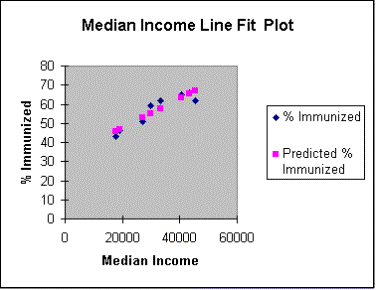
Note
the coefficients : The intercept is
31.72 and the slope is
0.00078 so we have the following equation:
Percent = 31.72 +
0.00078(Median Income)
We
used the default of 95% for the confidence level. Note the upper and lower 95% confidence limits appear in blue on
the above chart.
ASSIGNMENT: Do Exercises 13.58, 13.60, 13.75, 13.76
in your text.

